
Overview
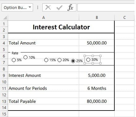
In this tutorial, you will learn, how to make a group box and add option button for excel form controls.
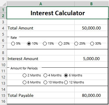
Below is the sheet, i’ll be using for interest calculator.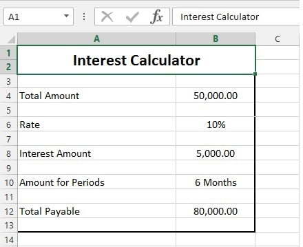
Need help with Guides & Tutorials?
Get a free strategy session with our experts — no commitment required.
Step 1:
We will use form controls. Form controls are advanced level features in excel that are hidden from normal users. So, we need to show developer tab in Ribbon. For that, we'll right click in the blank area.
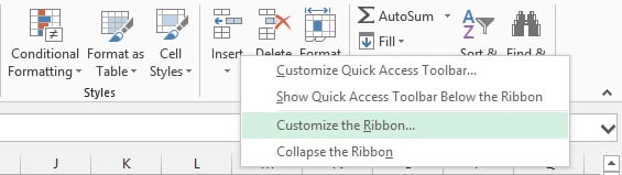
And select "Customize the Ribbon..." You'll see the following window dialog.
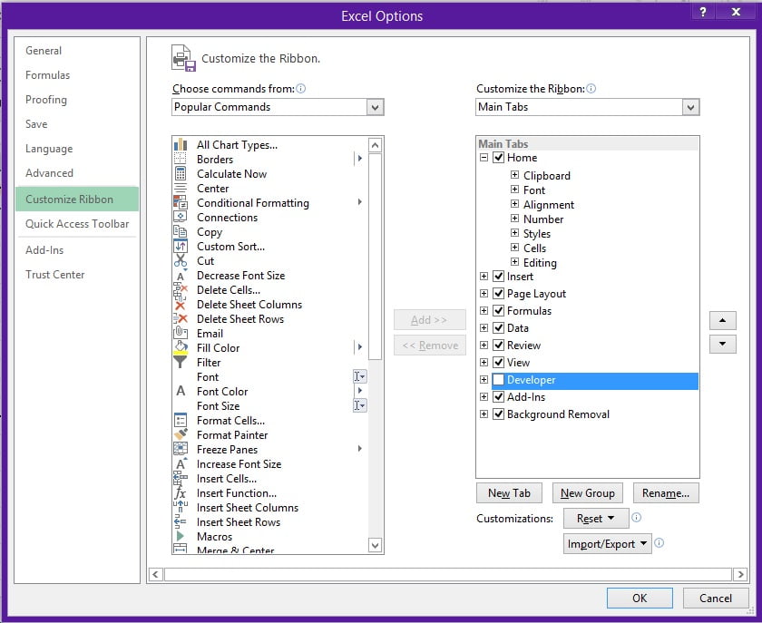
You'll find everything ticked except "Developer" option. Tick this option and Click "OK" to add Developer features to Ribbon.

Step 2:
Under Developer Tab, you'll find insert option, that'll be holding two types of controls.
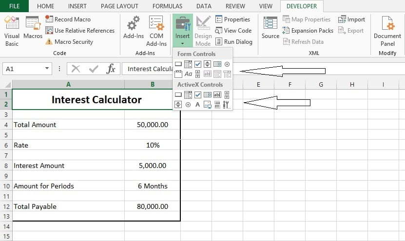
Form Controls are used in excel forms, while ActiveX Controls are used with Visual Basic. I'll use Form Controls here.
**HOW TO USE COMBO BOX FROM EXCEL FORM CONTROL**
I'll use Group options for "Rate" and "Amount of Periods". So, i'll remove the row holding "Rate". And insert two rows for Group Box.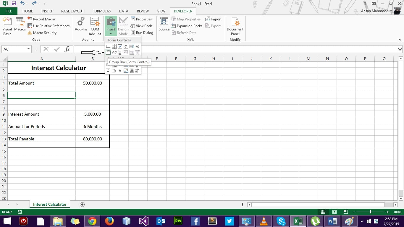
Select Group box, and Move cursor to Row 6. Press Alt and Click & Hold mouse button and drag it to row 6 and 7 under Column A & B.
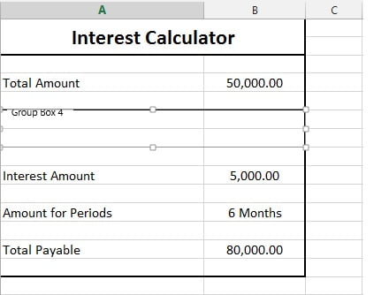
Change "Group box 4" Caption of group box by double tap on it and Write text to "Rate".
Step 3:
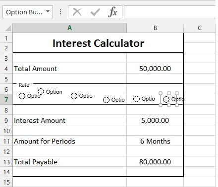
Now we need to add Option button from Form Controls again. So i'll select and insert them into Group box.
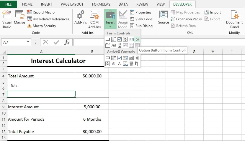
After Selecting Option Button from Form Control, Move mouse Cursor into Group Box, Press Ctrl and Draw with mouse button. It is the best practice and more professional to start from left side aligned.
Step 4:
Key steps and notes
To change the caption of Option box, Press Ctrl and Click on option to get focus and Click on Text to edit.
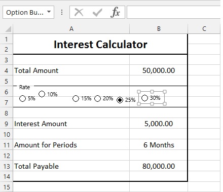
After changing caption of Option boxes, you need to check that clicking on one option box should diminish the other selection of option box. It means one option box should be selected at one time.
Step 5:
Now, you see the option boxes are not of same size. We can resize them equally by focusing and moving there edges with Mouse. But that is not so professional way to do as there will be some difference left. So we need to resize it using Format tool. Move cursor to any option button and get focus. Right click on it and select "Format Control". You'll get a window Dialog in front.
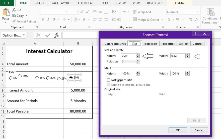
Note Height and Width of one Option button.
Step 6:
Now, Get focus of one option button and Press Ctrl and click on all Option buttons to select.
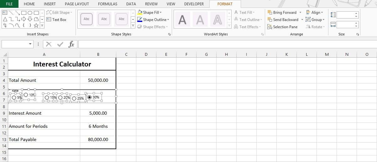
And Right click on "Format Object" option.
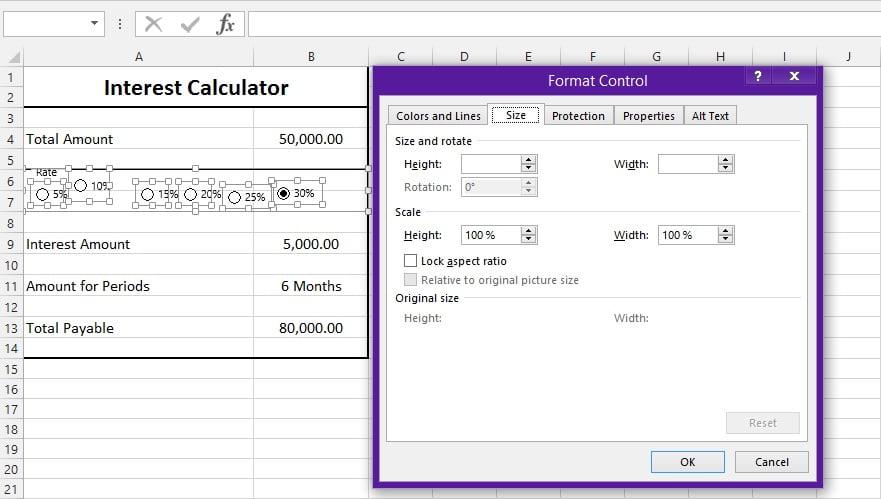
Enter those values you found in Step 5, in Height and Width. And you'll see all option buttons in same size.
Step 7:
We need to align all the option buttons. So, again i'll select all by selecting them by pressing Ctrl and Mouse click. And then Move to "Format" tab. And select "Aling Middle" in "Align" Option.
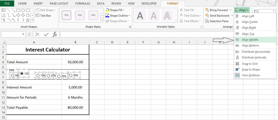
And then we'll relocate them with equal gaps in between them by selecting "Distribute Horizontally" in "Align" Option.
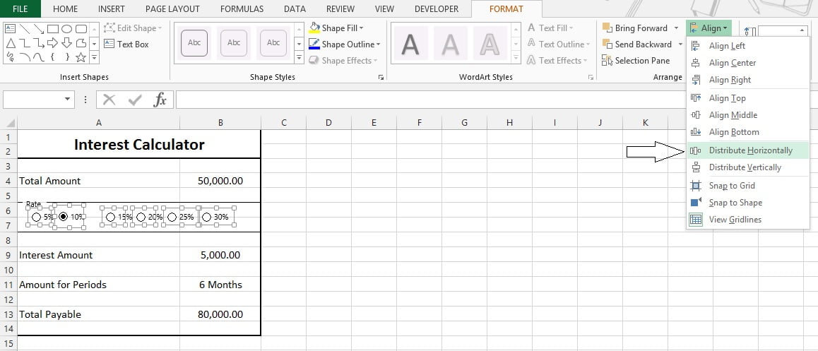
You'll get this group like
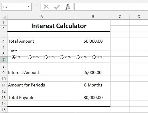
Step 8:
Same Steps to follow for "Amount for Periods". You'll get it like:
Final notes
Share your reviews in the comment section and let me know
How to do data validation in Excel
Overview
Data Validation helps us to make our Excel sheet error free. With data validation, we can define which data type cell can accept. We can also provide a list of values, in which we can select. Entering wrong value will prompt with an error. In this tutorial, we'll learn how to do data validation in Excel 2016.
Data Validation:-
We have a sheet with a table of data.
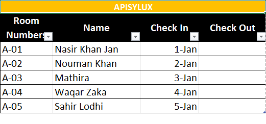
In the table above, These are just five entries. Suppose we have 1000 of entries like this in one table. And we are using that data for some calculations. A little mistake may give us wrong results. Suppose we have room numbers. We need it error free. We'll add data validation on room numbers column.
For that, You need a pre-occupied list of data. Verify that list is perfect and error free, all the values are right. Select the range of the cell on which you want to apply validation.
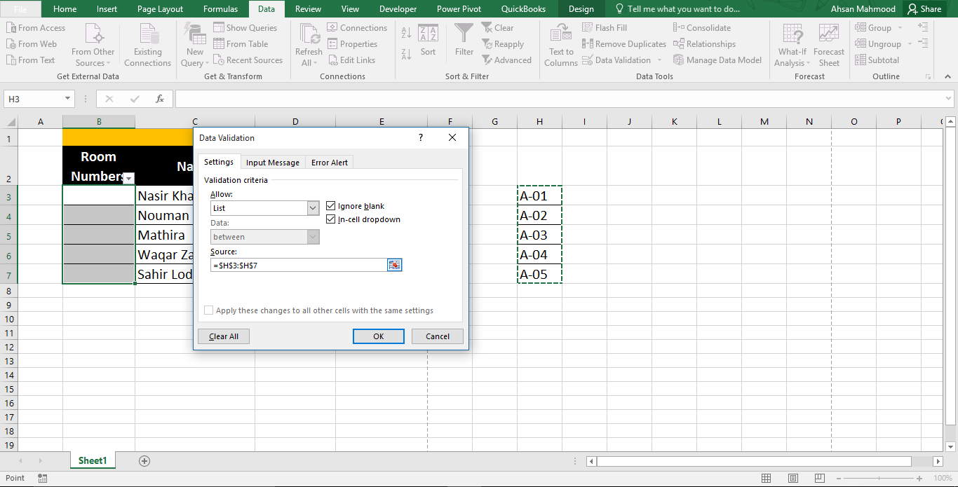
And in the menu ribbon, Go to "DATA" and select "DATA VALIDATION". You can use shortcut key for that. Select the range of cells, and Press "Alt+A+V+V". These shortcuts are hard to remember but practice makes everything perfect.
You will see a dialogue box as below in the picture.
Key steps and notes
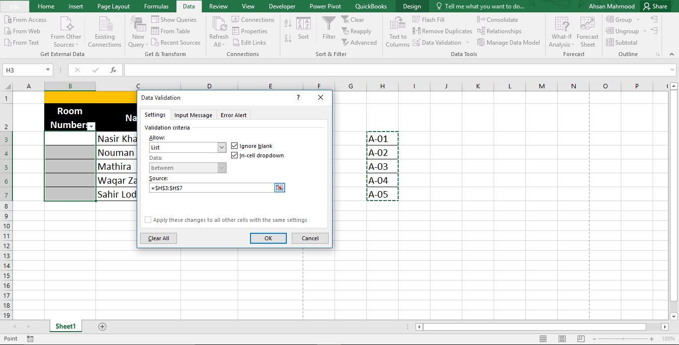
You'll see Validation criteria dropdown list. *These are all those options you can apply for validation." Select "List" among those options. And select the source data. Source data is the list of pre-occupied data that is verified as error free. Select the source range on the sheet.
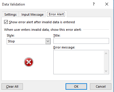
In the upper portion of dialogue box, You will see two more tabs.
Input Message
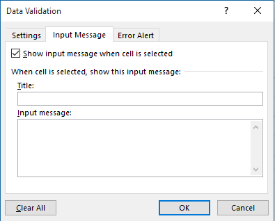
You can enter information about the cell in this tab. When cell is selected, information pops out for user ease.
Error Alert
Final notes
It facilitates with restriction about the wrong value. It will prompt if user will enter any wrong value and restricting to update the data in the cell.
After finishing, You will see that the cells in column of Room number is showing a dropdown arrow. Clicking on that one, you'll see verified list values. You have successfully applied data validation on Room number Column.


