ComboBox from Excel Form Control

Overview

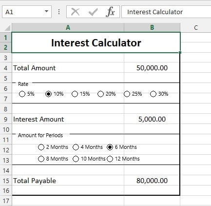
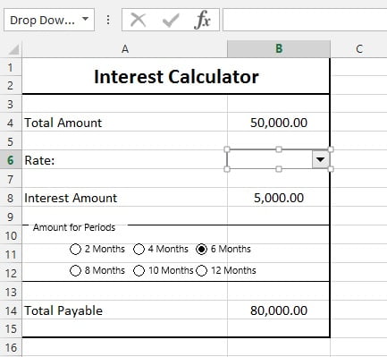
In this tutorial, you’ll learn how to use Combo Box form control in your excel sheet. We'll be using Interest Calculator for this purpose, as shown below:

Step #1:

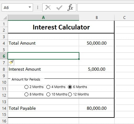
We'll replace "Rate group box" with Combo Box. So, we'll select Group box and press 'Del' button. Then, press ctrl and click on Radio Buttons to select them and press 'del'. we'll remove the rows 6 & 7 and Add one new row.

Step #2:

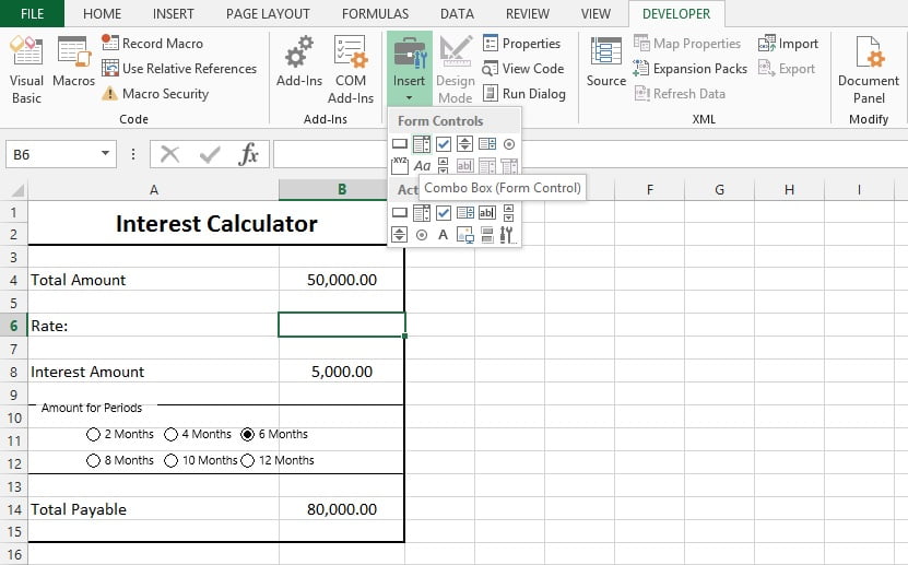
We'll insert the Combo Box in B6 box. For that we need to insert Combo Box from Insert in Developers Option.

Step #3:

Press alt and, Click and drag in B6 to draw Combo Box.

LEARN HOW TO APPLY DATA VALIDATION IN EXCEL

Step #4:

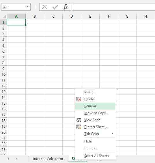
To add list of values, we need to list all the value on other sheet. And use that range in Combo Box. So, we'll create new Sheet with the name "Data" and list all the values of interest rates.

Key steps and notes

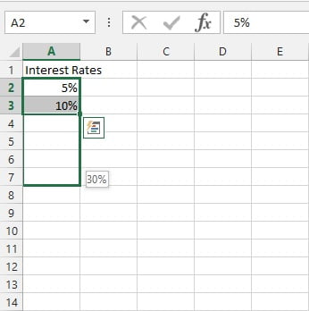
We'll enter two values with the difference of 5%. Select these two values and drag down to 5 cells. Excel will detect the difference and fill the values with the difference of 5% in each cell increasingly.

Step #5:

It's best practice to define name for ranges to select them. So, We'll select the cell ranges with values and go to "FORMULAS" ribbon tab. And select "Create from Selection".

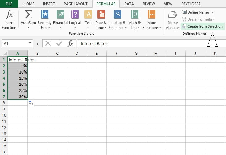
It'll pop out a dialog box to give you options to select naming box for the range.

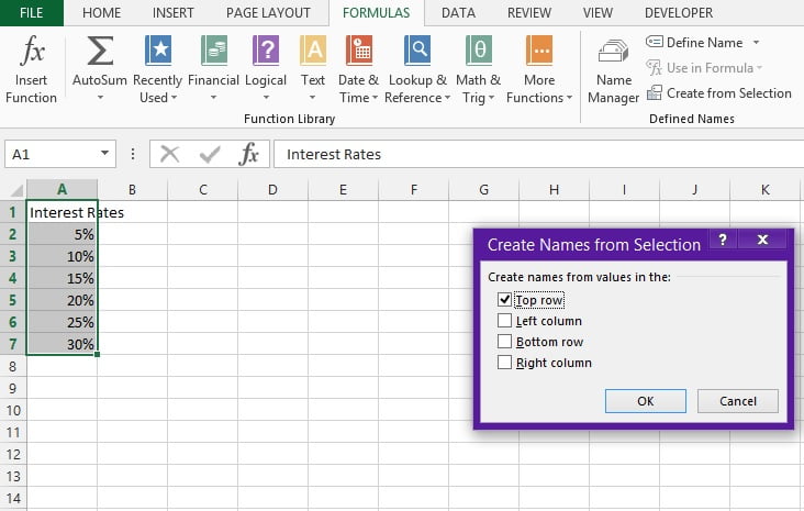
We have name to define range in the top row. So we'll select "Top row" and select Press OK.

Step #6:

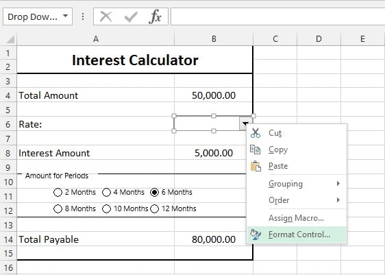
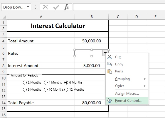
Now we have a defined name for the values of interest Rate. We'll go to "Interest Calculator" Sheet. Select Combo Box and go to Format Control.

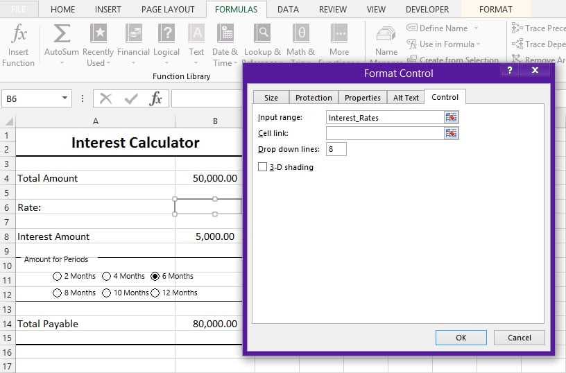
It'll give you dialog box to insert range of cells for the values. We'll insert the name defined for values.

I.e.: Interest_Rates

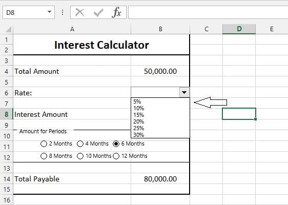
Press OK. Click on some other cell to remove selection focus of Combo Box. And then Check the Drop Down List, you'll see all the values of range entered on "Data" Sheet.

Final notes

Share reviews in comments.

Naming a cell range (the ComboBox input source)

Overview

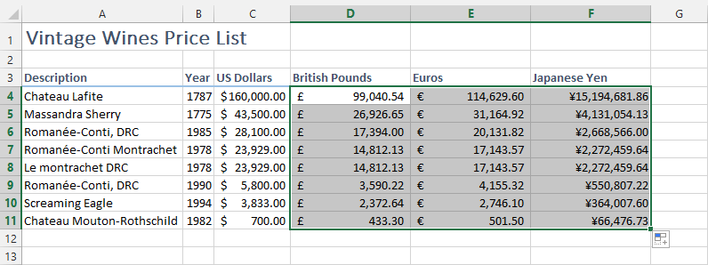
In this tutorial. We're going to set the Excel Range name for the cells in worksheet. Let's have a look on the worksheet i'll be using.

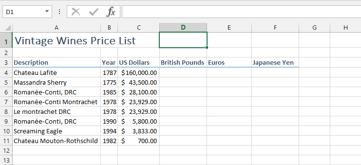
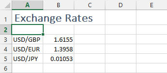
In this worksheet, we'll change the price of wines from US Dollars to British Pounds, Euros and Japanese Yen. I'll be using currency conversion rates in a table so the values will be used in this worksheet. Let's see the exchange rate table.

Step#1:

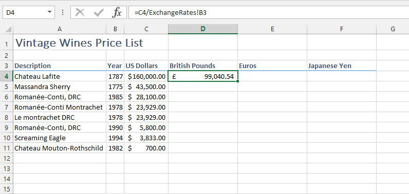
Let's calculate the currency amount in British Pounds for the "Chateau Lafite". So, we'll use the following way:

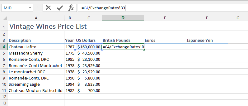
Where C4 is the reference to price in US Dollars and "ExchangeRates!B3" is the reference to conversion rate of USD to GBP. "ExchangeRates" is the name of the worksheet containing table of currency conversion rates. We'll get the following value in box.

Step#2:

Wouldn't it be nice if instead of "ExchangeRates!B3", it is something "=C4/USD_GBP". So it'd be completely clear that what formula is representing. This can be done by using Range Names. Range Names point to the value in a cell that can be used in formulas, constants and tables.

**LINK EXCEL WORKSHEET TO WORD DOCUMENT**

We're going to rewrite the formula. So i'll delete the existing formula.

Step#3:

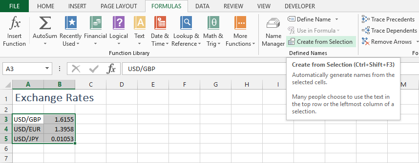
First of all, we'll create the names of the currency conversion rates. For that we'll select both columns in "ExchangeRates" worksheet. And we'll move to "Formulas" in Ribbon Tab and Select "Create from Selection".

Step#4:

A pop-up box will appear on the screen.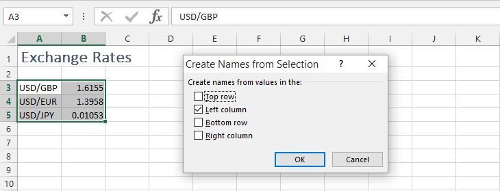

Key steps and notes

Select the "Left Column" and Click OK. So, it'll create the range names point to the values in Column B.

Step#5:

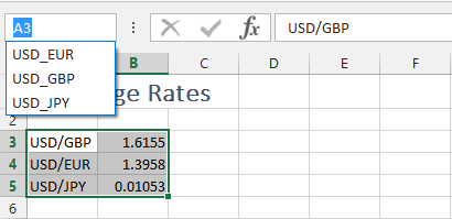
You can check the defined range names by clicking box in left up corner of worksheet table.

HOW TO DO DATA VALIDATION IN EXCEL

Step#6:

Now moving to the main Worksheet to apply the formula again. Again selecting box under "British Pounds", and applying formula:

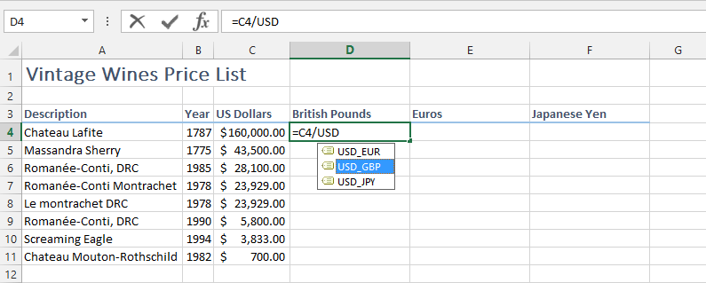
It'll give same value but with different Formula Description that is clearly understandable.

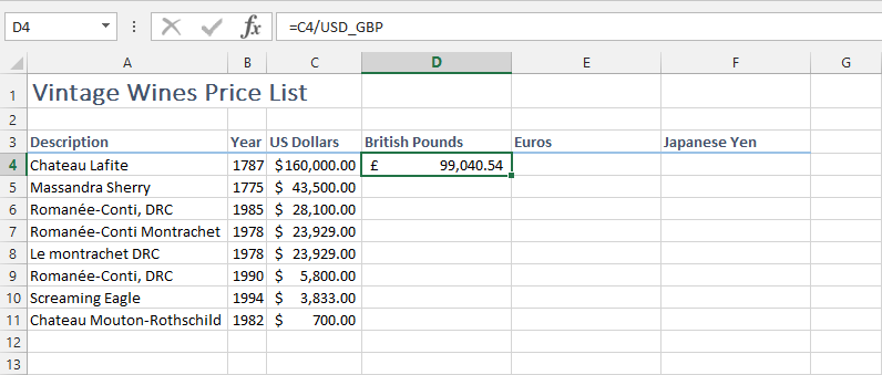
In the same way, we'll do for the Euros and Japanese Yen.

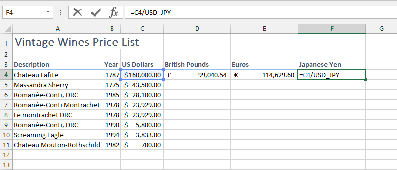
Step#7:

There is another way to get a list of range names to be used in formula or constants. For that you need to select box, write formula structure and go to "Formulas" in Ribbon Tab" and select "Use in Formula". It'll give a list of range names, so you can select one to use.

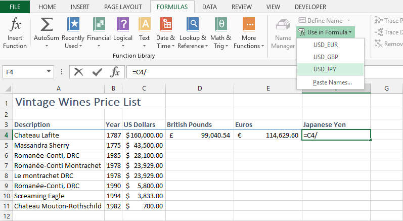
Step#8:

Select the three boxes, and drag them down to get the values of all the prices in currencies.

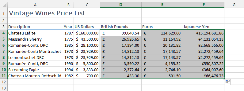
Final notes

In this way, we can define and use the range names in formulas. That makes it easier for user to understand the formula.

Share your reviews in the comment section.